Eclipse of WASP-189 b

Introduction

Warning

This tutorial does not use real CHEOPS data, only a realistic example data set. Don’t interpret any science results from this example!

The strength of some CHEOPS observations will come from the spacecraft’s ability to return to targets and repeatedly measure low signal-to-noise events until we can confidently detect small photometric features, like the depth of secondary eclipse of a hot exoplanet. This is the case for WASP-189 b, a very-hot Jupiter which orbits a bright A star (Anderson et al. 2018).

Sigma clipping

First, let’s import some packages we’ll need, including linea:

import numpy as np
import matplotlib.pyplot as plt
from scipy.stats import binned_statistic
from batman import TransitModel

from linea import JointLightCurve, Planet

# Load the transit parameters for WASP-189 b
p = Planet.from_name('WASP-189 b')

# Load the example light curve of WASP-189 b (built into the package)
lcs = JointLightCurve.from_example()

In the last line, we initialized a JointLightCurve object using the from_example method, which loads example (fake) data of four visits of WASP-189 b.

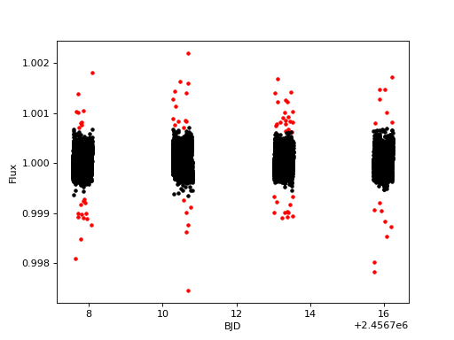
Then we sigma-clip the light curve – this removes outliers.

# Sigma clip the light curve to remove outliers
for lc in lcs:
    lc.sigma_clip_flux(sigma_upper=3, sigma_lower=3, plot=True)
    plt.show()

(Source code, png, hires.png, pdf)

Regression analysis

We assemble each indidiual visit’s design matrix by calling combined_design_matrix, which combines them into one big design matrix. We’ll also concatenate the design matrix of basis vectors with an eclipse model, computed by batman:

all_lcs = lcs.concatenate()

eclipse_model = TransitModel(p, all_lcs.bjd_time[~all_lcs.mask],
                             supersample_factor=3,
                             transittype='secondary',
                             exp_time=all_lcs.bjd_time[1]-all_lcs.bjd_time[0]
                            ).light_curve(p) - 1

X = np.hstack([
    lcs.combined_design_matrix(),
    eclipse_model[:, None]
])

Now X contains our “final” design matrix, consisting of the all of the basis vectors we can think of, and the eclipse model.

To do the linear regression, simply call the regress method:

r = lcs.regress(X)

The solution to the linear regression is stored in r. One neat measurement we can pull directly from the r object is the best-fit eclipse depth and its uncertainty. The transit model we intiailized in eclipse_model has a depth of 1 ppm, so the least squares weight for the eclipse (last) basis vector is the amplitude of the secondary eclipse in units of ppm. The eclipse depth and uncertainty are:

>>> print(f"Eclipse depth = {r.betas[-1] :.0f} ± {np.sqrt(np.diag(r.cov))[-1] :.0f} ppm")  
Eclipse depth = 77 ± 7 ppm

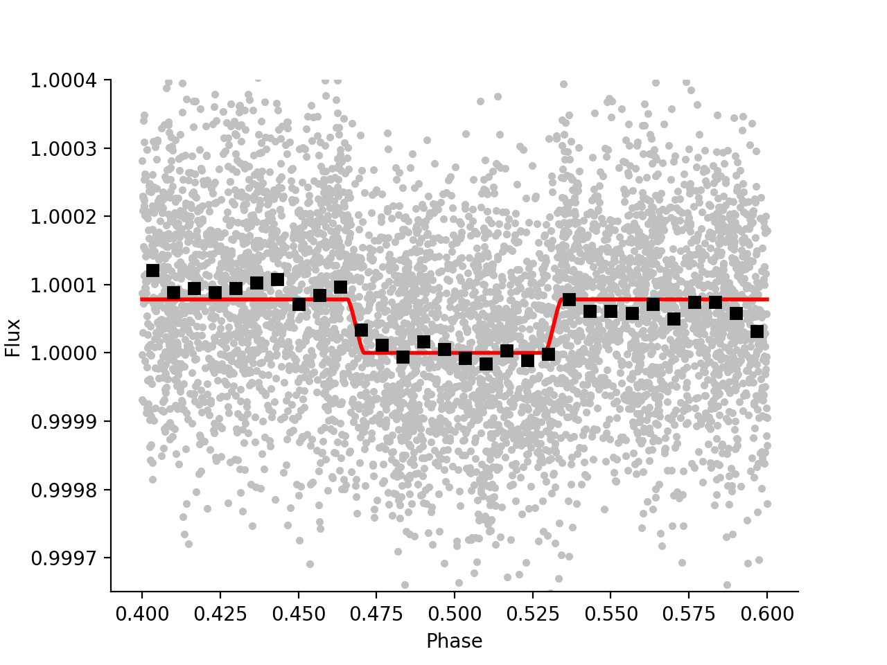
Finally, let’s plot the best-fit detrended light curve and eclipse model:

# Compute orbital phase for every time
phases = np.concatenate([lc.phase(p)[~lc.mask] for lc in lcs])
sort = np.argsort(phases)

# Compute the best-fit systematics model, without removing the eclipse
obs_eclipse = all_lcs.flux[~all_lcs.mask] / (X[:, :-1] @ r.betas[:-1])

# Compute the best-fit eclipse model
eclipse_model = X[:, -1] * r.betas[-1]

# Binned light curve:
bs = binned_statistic(phases[sort], obs_eclipse[sort], bins=30)
bincenters = 0.5 * (bs.bin_edges[1:] + bs.bin_edges[:-1])

# Create plot:
fig, ax = plt.subplots(figsize=(4, 3), sharex=True)

ax.plot(phases, obs_eclipse, '.', color='silver')
ax.plot(phases[sort], eclipse_model[sort] + 1, 'r', lw=2)
ax.plot(bincenters, bs.statistic, 's', color='k')

for sp in ['right', 'top']:
    ax.spines[sp].set_visible(False)
ax.ticklabel_format(useOffset=False)

ax.set(xlabel='Phase', ylabel='Flux',
       ylim=[0.99965, 1.0004])
plt.show()

(Source code, png, hires.png, pdf)

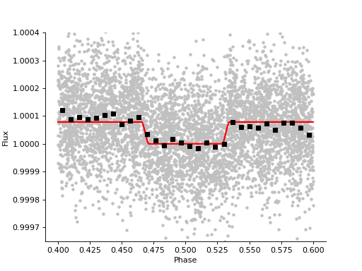
Note

The above plot is a simulated example light curve, not real CHEOPS observations. Do not make any conclusions about the planet from this fake dataset.

We can clearly see the ~80 ppm secondary eclipse which occurs when the planet is occulted by the star.